In the previous post, I wrote about a biography of Oliver Heaviside I had been reading. It is a biography, and not a technical treatise, but it does have end notes to some chapters with pages of maths. Maybe the author is more comfortable with maths that he is with the engineering application of it, so we have to allow that he might have omitted some important details.
My interest piqued, I also turned to my copy of “Life of Lord Kelvin” by Sylvanus Thompson.
Kelvin started life in 1824 as William Thompson. He did not become Lord Kelvin until 1892, but Kelvin is the name we know him by, so I will refer to him thus. He died in 1907.
The books shows us that in Heaviside and Kelvin’s early times, transmission lines were modelled as distributed series R and shunt capacitance. No Inductance!
Was it just that the significance of inductance was not understood at the time, or was it that the particular applications of transmission lines in those days had the character that line inductance was not significant. The Heaviside book does not tell us, but in the Lord Kelvin book we read:
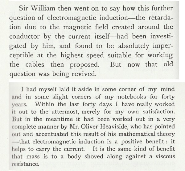
The “but now” in the above snippet from the book, appears to be when the telephone was introduced and greater bandwidth was required.
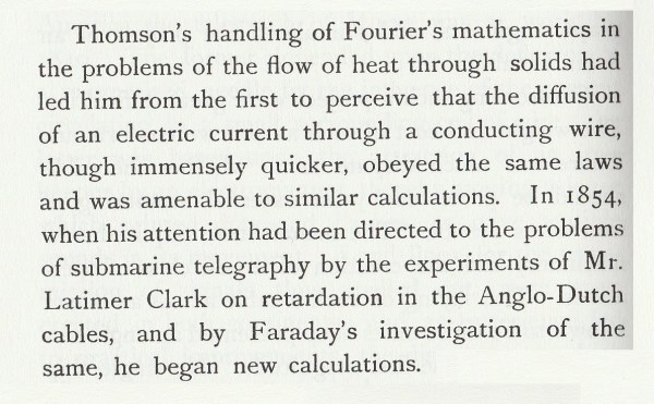
When inductance is ignored, then the transmission of a change in voltage down a line is analogous to the transmission of a change in temperature in a solid. This problem had been tackled and resolved by Fourier. Lord Kelvin specifically acknowledged Fourier.
From Life of lord Kelvin
In addition, we are led to believe that Heaviside stated that for analysis purposes, all the shunt capacitance of a transmission line such as a submarine cable could be modelled as concentrated at the centre. For practical purposes, he and his contemporaries seemed to have found that simplification justified. In 1850 overland telegraphy was well established, and by 1856 a large number of short submarine cables were in service.
What could be done to increase the speed of a cable that behaved like a hot poker (Fourier)? In looking at this on the simulator, I have chosen a very simple Morse code message: the one, which just a few years ago, I used to hear from my mobile phone. “SMS”. As most people who know very little of Morse code know, “S” is three dots. We know this from the Morse for “SOS”. “M” is two dashes. My reasons for choosing this as a test message rest both with its familiarity, and the fact that it is exceedingly easy to generate with Pulse generators in the simulator.

My method (This is MY method: there is no hint that Heaviside or Kelvin ever did this.) is to write out my model circuit, and then look at its response in the frequency domain. After making some changes to the model in an attempt to improve this, I look at how it might come up in the time domain. For my models I have chosen my time scale completely arbitrarily. As an artefact of one of my “mucking around” sessions, I have different time scales for my frequency and time domain analyses. Don’t you worry about this. You can do all this with whatever time scale you wish. Just change the capacitor values and the speed of the pulses accordingly.
Before I start, a little note on the way speed is characterized in Morse. Heaviside and Kelvin had not heard of Baudot at this time! (Modern measure of symbol rate is the “Baud”. Computer buffs please note that this is pronounced “Bode”. Named after Baudot, of course.) In the paragraph that follows, The two symbols are referred to as “dit” and “dah”. I believe that these names would have arisen when morse came to be used for radio communication. They represent the sounds of the symbols when heard on a receiver with a beat frequency oscillator. “Dot” and “Dash” in Heaviside and Kelvin’s day as the symbols were seen on a paper tape.
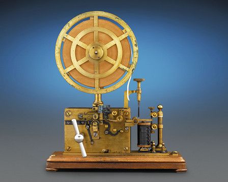
Paper tape inker for recording Morse code traffic. The tape is moved by a clockwork machanism. The received signal appears as dots and dashes on the tape.
From: http://en.wikipedia.org/wiki/Morse_code
“The speed of Morse code is typically specified in “words per minute” (WPM). In text-book, full-speed Morse, a dah is conventionally 3 times as long as a dit. The spacing between dits and dahs within a character is the length of one dit; between letters in a word it is the length of a dah (3 dits); and between words it is 7 dits. The Paris standard defines the speed of Morse transmission as the dot and dash timing needed to send the word “Paris” a given number of times per minute. The word Paris is used because it is precisely 50 “dits” based on the text book timing.
Under this standard, the time for one “dit” can be computed by the formula:
T = 1200 / W
Where: W is the desired speed in words-per-minute, and T is one dit-time in milliseconds.”
Here is a model of a submarine cable. The model is built according to Heaviside’s simplification: that is, it has all the capacitance lumped in the middle.
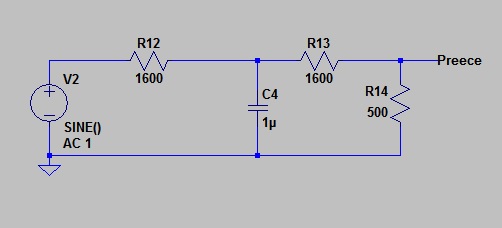
I have called the signal on the output “Preece” as this represents a badly designed system (See last post for information about Preece)
Telegraphers had noticed that when a marine cable developed a fault (resistance in shunt), the speed at which it could be worked increased. The problem with such faults (caused by salt water ingress, I suppose) is that they inevitably got worse. Heaviside said that if only one could have a low resistance across the line that stayed fixed (did not get worse), then the speed of the circuit would be permanently increased. He proposed a resistance of a value as low as a thirty second of the series resistance of the cable.

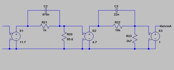
Here is a frequency domain representation of the performance of the Preece and the Heaviside cable.
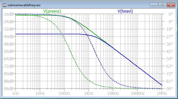
The Heaviside cable had lots more attenuation, but a decade more bandwidth. For my time-domain simulations, I am going to assume “Double Current Working, and a sensitive balanced relay on the receiving end. I am assuming that the relay acts like a zero crossing detector. I have added DC offsets just for display so that the traces are separated.
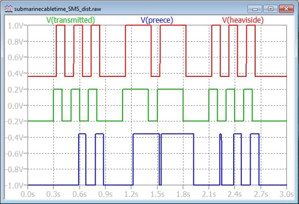
Note that I have chosen the time scale in the simulation so that the Heaviside trace is good, but the Preece trace is not. I left the time scale the same for all following time-domain simulations.
On all three traces, “Mark” is positive, and “Space” is negative. You can see that the signal on the contacts of the balanced relay in the Heaviside case is a faithful reproduction of what was transmitted. Easily read as “SMS” by the operator.
The “Preece” signal, however suffers from severe Telegraph Distortion. Telegraph Distortion was the term that used to enjoy official sanction is Standards as the name for distortion of a two state signal in which the relative timing of the transitions deviates from what is sent.
The first dot is missing entirely, as the sending key has not had time to remove the negative charge on the line capacitance due to the proceeding extended Space state. The two dashes of the letter “M” would be hardly recognized as such, and the three dots from the second “”S”, sent where the original bias on the line has been neutralized a little, is not much better than the first group of three.
Heviside had done a good job of improving the performance of this marine cable. The installation of a shunt resistor at the half-way mark in the cable must have been a bothersome thing, though. Best to eliminate that. So I had a crack at it myself. I have an advantage over Heaviside: the spice simulator. My approach was to see what sort of compensator I could add at the receiving end of the line to get the same effect. I started in the frequency domain. In the first instance, I restricted myself to components that would have been available in Heaviside’s day. (NO op-amps!)
Here is my first effort.

Here is how this comes up against Preece and Heaviside in the frequency domain.

You can see that the “Richard” model has a frequency response that is almost exactly coincident with the “Heaviside” one. At this point I am going to stop showing the time domain responses for the receiving of “SMS”, as they are all the same except the “Preece” one.
The Richard circuit model worked as well as Heaviside’s, and it would seem that it would have been much more convenient to place a resistor and inductor across the line at the receiving end, than to install and maintain a resistor under the sea.
The fact that a shunt inductor is of value is of interest in the light of a subsequent event as well.
A question arose: what if the simplification of the cable model by placing all the capacitance in the middle, although shown to be valid for Heaviside’s purposes, is not valid for my process of tweaking my compensation with frequency domain purposes and then testing in the time domain?
I repeated all the above model runs with a cable model consisting of cable resistance divided into four equal parts and three capacitances to ground from the junctions. The results were identical, although I had to change the value of resistance end inductance for my terminator. It did not seem to be necessary to try extending the model further towards fully distributed capacitance.
I decided to go a little further. What if I modelled a compensator without the restrictions that the components must have been available to Heaviside? It happens that this gives us a start to an approach that when followed through gives us a scheme that would have been realizable in Heaviside or Kelvin’s day.
I decided to try high frequency boost. This requires voltage gain, which was not available to Heaviside, but follow me like a leopard, and we will see what we could have offered him.
The circular symbols are voltage controlled voltage sources (idealized amplifiers). The number to the right, and below the symbol is the voltage gain.
I won’t cover the process for arriving at this compensator circuit here (although I will account for it if asked).
Here is the frequency response of the compensator.

As with all these plots, the solid line is amplitude, dotted line is phase.
Here is the frequency response of the whole shooting match with compensator included.
Almost 20 dB more gain than the Heaviside scheme of the mid cable shunt resistor, and a little bit of extra bandwidth. The output from the balanced relay is identical. The extra gain might be important on a very long cable where signal strength at the receiving end might not quite meet the balanced relay requirements.
Let us look at the time domain response of this compensator and consider what it is doing for our long, high capacitance submarine cable. What I have done here is put the compensator first: that is at the transmit end of the cable.
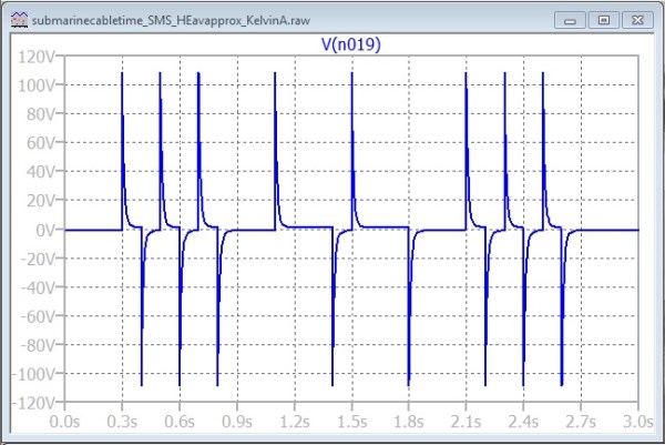
What we see here is the SMS waveform with an amplitude of about 2 volts, and superimposed, 110 volt spikes accentuating the transitions or edges in the data stream. It is easy to see in this time domain representation what the compensator is doing for the cable. At the beginning of each positive pulse, the large spike adds charge to the cable capacitance, and at the end of each pulse, a negative going spike removes that charge again.
After the first trans-Atlantic cable was laid, it was destroyed when one of the engineers set up an induction coil that imposed 2kV impulses on the line. I have only read about this in de-technicalized writing aimed at non-electronic engineers. Such writing leaves the interested reader guessing as to what had really been going on. Perhaps my compensator gives a clue. Perhaps attempts were made to generate a waveform like the above to increase the signalling rate. Perhaps it appeared that if 110 volts was good, then 2kV would be better. Whatever the reasoning, the 2kV was too much for the gutta percha insulation of the day, and the cable was destroyed.
It occurred to me that if this waveform, that was derived from my circuit model that could not have been represented by available hardware in the 1850s has the desired effect, then maybe we can introduce short pulses to quickly charge and discharge the cable capacitance without necessarily following the waveform exactly.

This graph shows a waveform presented to the send end of the cable (in red). This could have been generated by some mechanical momentary action relay that switches in the higher voltage momentarily at each transition. Nothing here that could not have been done in the 1850s.
The voltage of the spikes is only eleven times that of the raw data (as opposed to 55 times from the linear model). However the height and width of the spike are adjusted to have about the same impact on the charge of the line capacitance. The receive end in this model has no sort of compensator or special termination: just the model of the balanced relay (zero crossing detector). The result is a perfect Morse rendition with a little delay (green).
A little more Heaviside to come.